A couple of weeks ago, we released bcov, a tool for efficient binary-level coverage analysis via static instrumentation. The tool supported only two operation modes, namely, patching and coverage reporting. Today, we add another operation mode that dumps various program graphs, like the CFG and dominator trees, for a given function in the binary.
This neat feature can be useful in its own right. For example, we heavily relied on visualizing these graphs at various stages during the development of bcov itself. In this article, we first show how this mode can be used and then describe the generated program graphs.
Usage example
Consider the binary gas which is distributed together with our sample binaries.
For the sake of example, we will choose the function string_prepend.part.5.
It is small but still contains an interesting number of basic blocks.
To dump its program graphs, you can simply issue,
bcov -m dump -i gas -f "string_prepend.part.5"
This command should produce five DOT files in your current directory.
To visualize these files, we recommend the interactive viewer xdot.
The raw DOT files are provided here for convenience.
They are named after the address of the selected function as follows:
- func_4e6070.cfg.dot. The CFG of the function.
- func_4e6070.rev.cfg.dot. Similar to the CFG but with all edges reversed.
- func_4e6070.pre.dom.dot. Predominator tree.
- func_4e6070.post.dom.dot. Postdominator tree.
- func_4e6070.sb.dom.dot. Superblock dominator graph.
The first two graphs are probably familiar to you already. However, understanding the remaining graphs might require further reading. The definitive resource is the original work that we implemented in bcov. However, the summary provided in section 3 of our paper should be sufficient.
Graphs described
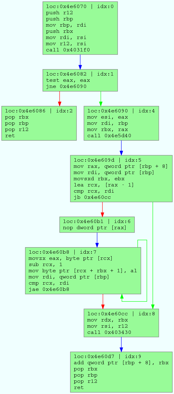
We start with the CFG below. Each basic block is marked with its address (address of first instruction) and a unique identifier within the function. Unconditional edges are blue colored. Conditional edges can be either green for the taken edge or red for the fall-through edge.
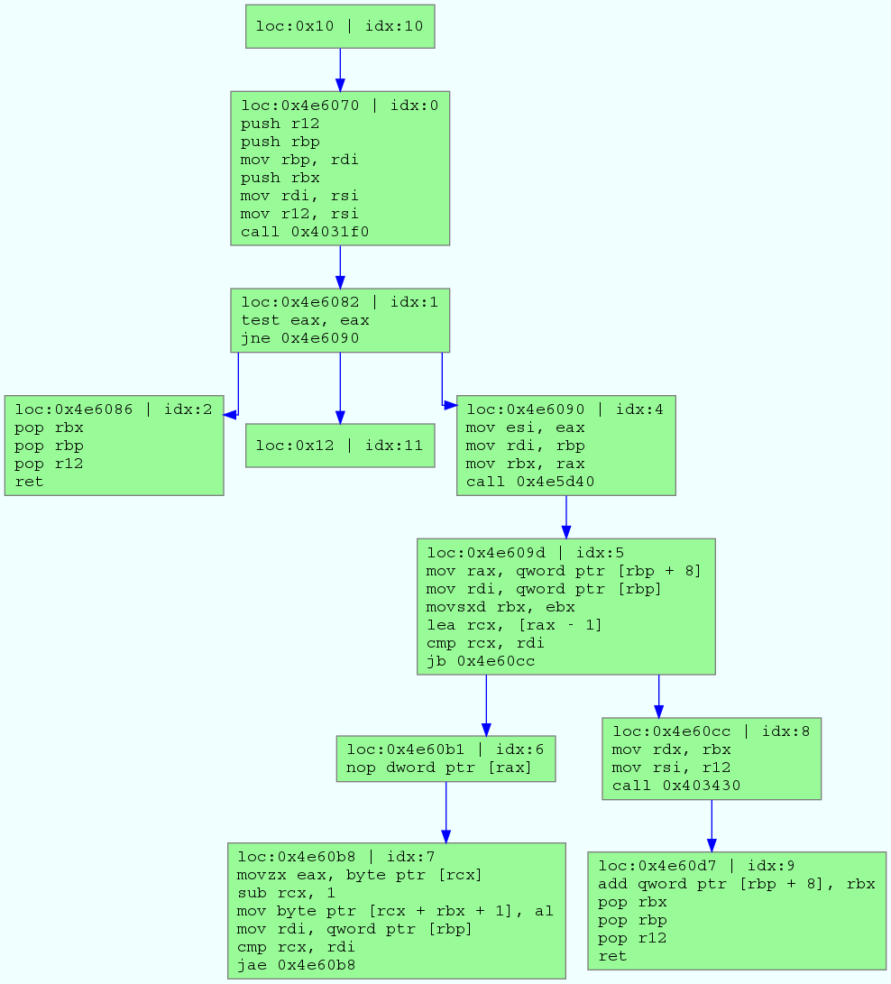
We move to the predominator tree. It is rooted in the virtual entry node. An edge between basic blocks A -> B means that A predominates B. Simply put, B can not be visited without first visiting A. For example, BB8 (i.e., it has idx 8) must be visited before visiting BB9. This dominance relationship enables us to substantially reduce the required number of instrumentation probes since covering a particular BB implies that all of its predecessors in the predominator tree are also covered.
The predominator tree is useful but we can still do better. First, we merge the predominator and postdominator trees in a dominator graph. Then, we identify the strongly-connected components (SCCs) in the latter graph to construct the superblock dominator graph (SDG). Each SCC represents a superblock that contains at least one basic block as shown below.
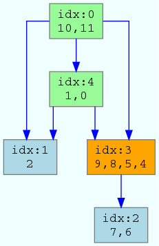
The instrumentation policies implemented in bcov are based on the resulting SDG. In the leaf-node policy, we only instrument the leaf nodes of the SDG (light-blue colored), namely, SB1 and SB2. SB1 consists of a single basic block, BB2. However, SB2 offers more flexibility to choose between BB6 and BB7. We leverage this flexibility in bcov to select the BB that incurs minimal overhead.
A test suite that covers all leaf nodes would also achieve 100% code coverage. Should you insist on a coverage target that ambitious, then the leaf-node policy is all that you need. However, engineers in practice will have to make compromises since software testing is costly. Additionally, a test suite achieving 100% code coverage is not necessarily more effective (i.e., detects more bugs) than a test suite that achieves, for example, only 80% coverage.
In such settings, the leaf-node policy might not be adequate since it may lose coverage data. The problem is that some superblocks might be visited in the CFG while bypassing all of their children in the SDG. We refer to such superblocks as critical. They are orange-colored by bcov like SB3.
The any-node policy solves this problem by instrumenting critical superblocks, in addition to the leaf superblocks instrumented in the leaf-node policy. That is, bcov would instrument one additional BB among the four in SB3. You can check that for any input, it is now possible to precisely identify the set of covered basic blocks in function 'string_prepend.part.5'. Such precision would require instrumenting only 3 BBs among a total of 10 BBs in this particular function.
I'm interested in your take on this piece. Please reach out by opening an issue in this repository.